# Load pacakges ---------------------------------------------------------------

library(SimCorMultRes)
library(MASS)
library(ggplot2)
library(ggExtra) # for marginal plots
library(e1071)
library(sn) # for skewed normal distributionIntroduction
The Normal to anything (or NORTA) is a sampling approach that allows the generation of multivariate data with a known rank correlation structure and arbitrary marginal distributions. For example, you could generate 2 variables \(X_1\) and \(X_2\) with a given rank correlation and beta marginal distributions. The only requirement is that the target marginal distributions need to be continuous distributions with a known (inverse) cumulative distribution function.
Learn by coding
For this topic we will need a few packages:
The NORTA approach can be summarized in three steps:
- Sample a data matrix \(X_{n \times p}\) from a Multivariate Normal distribution with target correlation structure
- Transform the distributions of the individual variables \(x_j\) for \(j = 1, \dots, p\) (the marginal distributions) to a uniform distribution by applying the normal CDF to \(X\) (in R
pnorm()) - Transform the uniform marginals to any continuous target distributions by applying the inverse CDF of the target distribution (usually implemented in R by a
qtarget()function, for example,qbeta)
1. Sample from a multivariate normal distribution
First, we sample 1000 observations from a multivariate normal distribution with four correlated variables (\(\rho = .7\)).
# 1. Sample from multivariate normal distribution -----------------------------

# Set the seed
set.seed(20210422)

# Fix parameters
n <- 1e3 # smaple size
p <- 2  # number of variables
mu <- rep(0, p) # vector of means
Sigma <- matrix(.7, nrow = p, ncol = p); diag(Sigma) <- 1 # correlation matrix

# Sample Multivariate Normal data
X <- mvrnorm(n = n, mu = mu, Sigma = Sigma)
We can then plot a scatterplot of \(X_1\) and \(X_2\) to study their multivariate distribution and make the marginal plots visible.
# Plot the multivariate distribution (scatterplot)
X_scatter <- ggplot(data.frame(X), aes(x = X1, y = X2)) +
      geom_point()

# Add marginals of X
ggMarginal(X_scatter, type = "histogram") 
We can now transform the marginal distributions of the \(x\)s to any target continuous distribution.
2. Transform normal marginals into uniform
For example, consider transforming the marginals to a beta distribution.
First, we compute the values of the normal cumulative distribution function (pnorm()).
# 2. Transform marginals to a uniform distribution -----------------------------

# Transform to uniform distribution (apply normal CDF to X)
U <- pnorm(X)

# Make scatterplot
U_scatter <- ggplot(data.frame(U), aes(x = X1, y = X2)) +
      geom_point()

# Add marginals of U
ggMarginal(U_scatter, type = "histogram") 
3. Transform uniform marginals into anything
Then we compute the quantiles corresponding to the resulting cumulative probabilities based on the target marginal distribution using the qbeta() function.
# 3. Transform marginals to anything with a (inverse) CDF ----------------------

# > 3.1 Beta -------------------------------------------------------------------

# Transform to a beta distribution
X_beta <- qbeta(U, shape1 = .5, shape2 = .5)

# And visualize
X_beta_scatter <- ggplot(data.frame(X_beta), aes(x = X1, y = X2)) +
      geom_point()
ggMarginal(X_beta_scatter, type = "histogram") 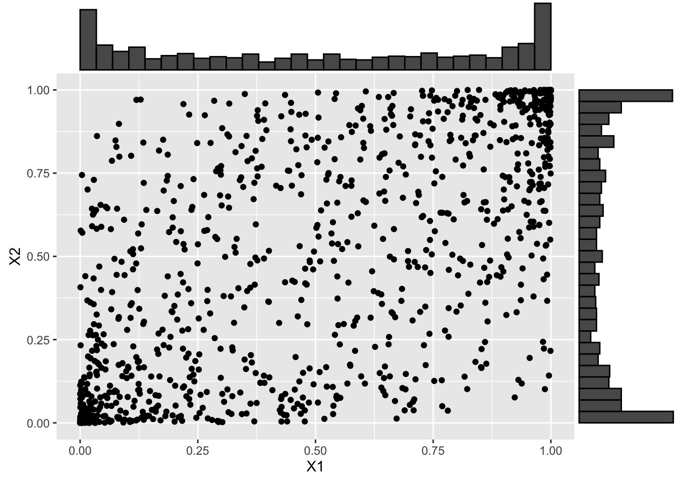
As another example, consider transforming the marginal to a highly skewed T distribution.
# > 3.2 Skewed-t distribution --------------------------------------------------

# Define the target skewness and kurtosis
sk <- -2
kt <- 10

# Define direct parameterization for the skew-t (ST) distribution
cpST <- c(0, 1, sk, kt)
dpST <- cp2dp(cpST, family = "ST")

# Transform to Skew-t (apply target inverse-CDF to X)
X_st <- apply(U, 2, qst, dp = dpST)

# And visualize
X_st_scatter <- ggplot(data.frame(X_st), aes(x = X1, y = X2)) +
      geom_point()
ggMarginal(X_st_scatter, type = "histogram") 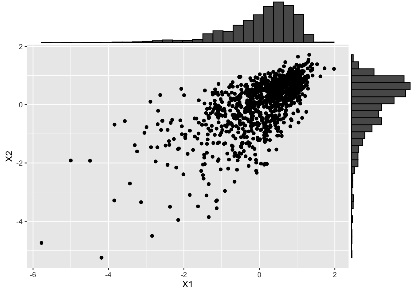
3.1 Preserved multivariate relationships
Upon generating the multivariate data \(\mathbf{X}\), the association between the two variables \(X_1\) and \(X_2\) is determined by the correlation coefficient \(\rho\) that we used in the mvrnorm() call. This coefficient expresses the linear dependence between the two variables which is not preserved when non-linear transformations are applied to the marginals (which we use). However, the NORTA approach does preserve rank correlations between the variables. In the following code, we compute the Pearson correlation (linear dependency), and the Spearman and Kendall’s correlations (rank correlations) for the original data, and all other transformations.
# Collect all sampled datasets
dats <- list(X = X, U = U, skewt = X_st, beta = X_beta)

# Compute all types of correlation on all datasets
round(
      data.frame(
            Pearson = sapply(dats, function(i) cor(i, method = "pearson")[1,2]),
            Spearman = sapply(dats, function(i) cor(i, method = "spearman")[1,2]),
            Kendall = sapply(dats, function(i) cor(i, method = "kendall")[1,2])
      ), 3
)
Pearson Spearman Kendall
X 0.684 0.666 0.476
U 0.667 0.666 0.476
skewt 0.663 0.666 0.476
beta 0.644 0.666 0.476As you can see, the NORTA sampling approach allows us to easily sample dependent multivariate data with arbitrary marginal distributions and known target (rank) correlations.
3.2 Discrete distributions
One can be tempted to use any marginal distribution, even discrete distributions. However, the rank correlation is not preserved when this marginal transformation is applied. Consider for example transforming the marginals to Poisson distributions:
# > 3.3 Poissan distribution ---------------------------------------------------

# Transform to poissan (apply target inverse-CDF to X)
X_pois <- qpois(U, lambda = 2)

# And visualize
X_pois_scatter <- ggplot(data.frame(X_pois), aes(x = X1, y = X2)) +
      geom_point()
ggMarginal(X_pois_scatter, type = "histogram") 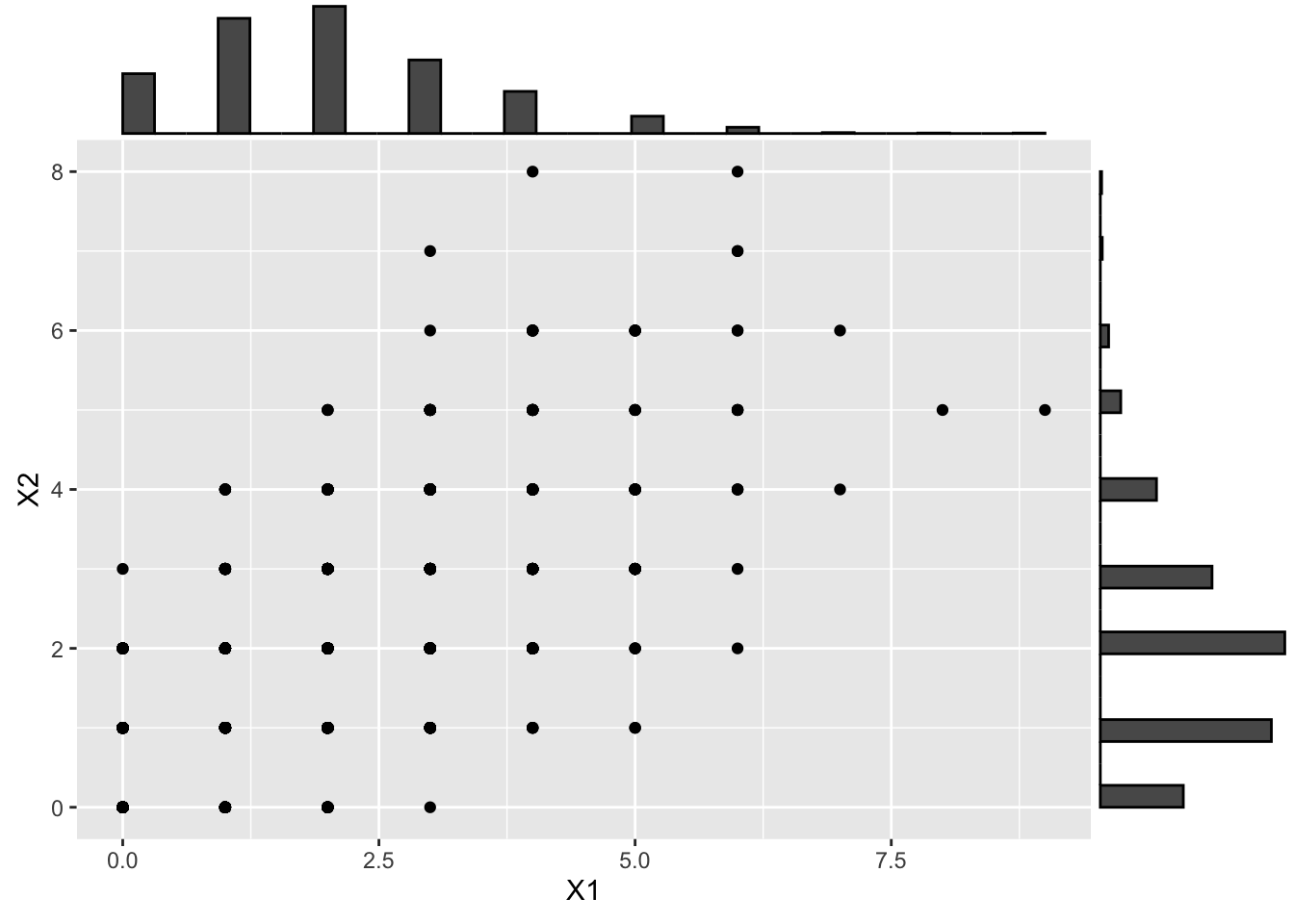
or to binomial distributions
# > 3.4 Binomial distribution ---------------------------------------------------

# Transform to binomial
X_binom <- qbinom(U, size = 6, prob = .2)

# And visualize
X_binom_scatter <- ggplot(data.frame(X_binom), aes(x = X1, y = X2)) +
      geom_point()
ggMarginal(X_binom_scatter, type = "histogram") 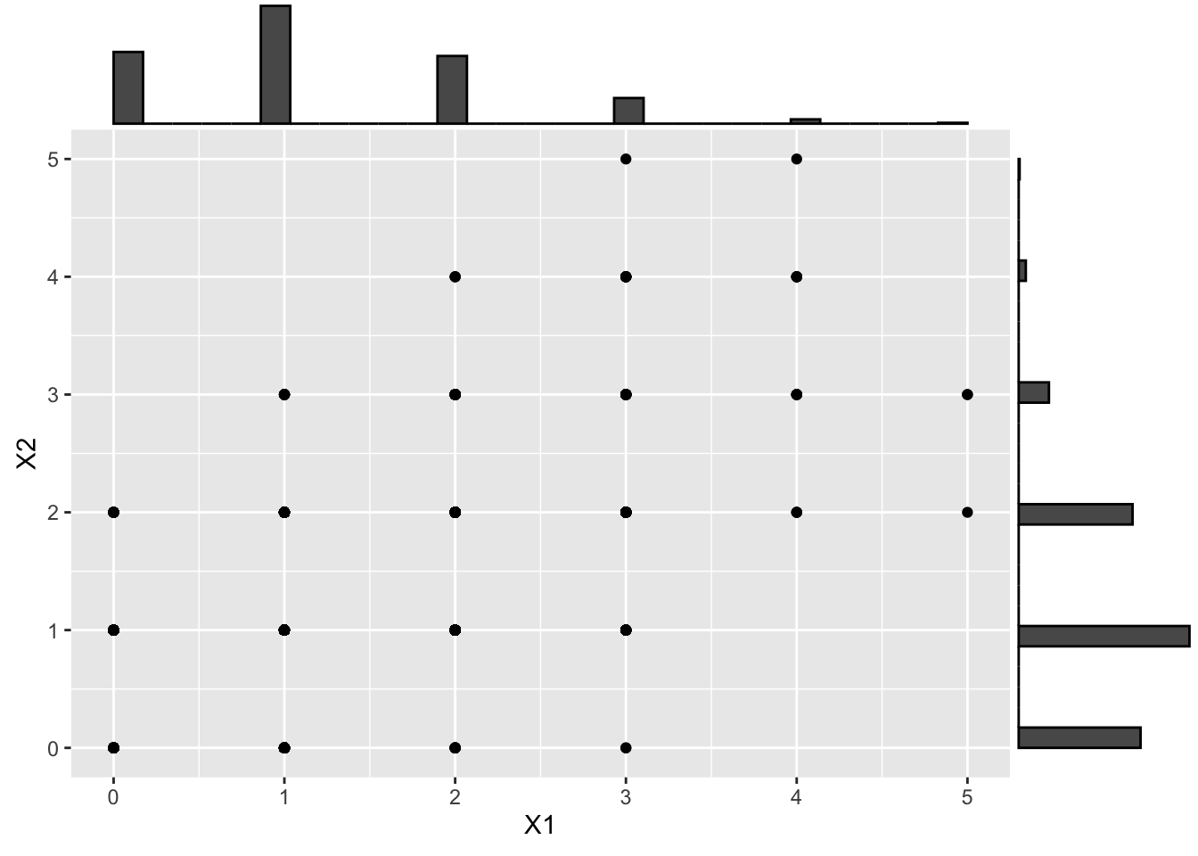
if you check again both the linear and rank correlations you will notice that both have been impacted by these transformations:
# Add the other datasets
dats <- list(
            X = X,
            U = U,
            skewt = X_st,
            beta = X_beta,
            poissan = X_pois,
            binomial = X_binom
)

# Compute all types of correlation on all datasets
round(
      data.frame(
            Pearson = sapply(dats, function(i) cor(i, method = "pearson")[1,2]),
            Spearman = sapply(dats, function(i) cor(i, method = "spearman")[1,2]),
            Kendall = sapply(dats, function(i) cor(i, method = "kendall")[1,2])
      ), 3
)
Pearson Spearman Kendall
X 0.684 0.666 0.476
U 0.667 0.666 0.476
skewt 0.663 0.666 0.476
beta 0.644 0.666 0.476
poissan 0.644 0.635 0.535
binomial 0.620 0.605 0.535TL;DR, just give me the code!
# Load pacakges ---------------------------------------------------------------

library(SimCorMultRes)
library(MASS)
library(ggplot2)
library(ggExtra) # for marginal plots
library(e1071)
library(sn) # for skewed normal distribution

# 1. Sample from multivariate normal distribution -----------------------------

# Set the seed
set.seed(20210422)

# Fix parameters
n <- 1e3 # smaple size
p <- 2  # number of variables
mu <- rep(0, p) # vector of means
Sigma <- matrix(.7, nrow = p, ncol = p); diag(Sigma) <- 1 # correlation matrix

# Sample Multivariate Normal data
X <- mvrnorm(n = n, mu = mu, Sigma = Sigma)

# Plot the multivariate distribution (scatterplot)
X_scatter <- ggplot(data.frame(X), aes(x = X1, y = X2)) +
      geom_point()

# Add marginals of X
ggMarginal(X_scatter, type = "histogram")

# 2. Transform marginals to a uniform distribution -----------------------------

# Transform to uniform distribution (apply normal CDF to X)
U <- pnorm(X)

# Make scatterplot
U_scatter <- ggplot(data.frame(U), aes(x = X1, y = X2)) +
      geom_point()

# Add marginals of U
ggMarginal(U_scatter, type = "histogram")

# 3. Transform marginals to anything with a (inverse) CDF ----------------------

# > 3.1 Beta -------------------------------------------------------------------

# Transform to a beta distribution
X_beta <- qbeta(U, shape1 = .5, shape2 = .5)

# And visualize
X_beta_scatter <- ggplot(data.frame(X_beta), aes(x = X1, y = X2)) +
      geom_point()
ggMarginal(X_beta_scatter, type = "histogram")

# > 3.2 Skewed-t distribution --------------------------------------------------

# Define the target skewness and kurtosis
sk <- -2
kt <- 10

# Define direct parameterization for the skew-t (ST) distribution
cpST <- c(0, 1, sk, kt)
dpST <- cp2dp(cpST, family = "ST")

# Transform to Skew-t (apply target inverse-CDF to X)
X_st <- apply(U, 2, qst, dp = dpST)

# And visualize
X_st_scatter <- ggplot(data.frame(X_st), aes(x = X1, y = X2)) +
      geom_point()
ggMarginal(X_st_scatter, type = "histogram")

# Collect all sampled datasets
dats <- list(X = X, U = U, skewt = X_st, beta = X_beta)

# Compute all types of correlation on all datasets
round(
      data.frame(
            Pearson = sapply(dats, function(i) cor(i, method = "pearson")[1,2]),
            Spearman = sapply(dats, function(i) cor(i, method = "spearman")[1,2]),
            Kendall = sapply(dats, function(i) cor(i, method = "kendall")[1,2])
      ), 3
)

# > 3.3 Poissan distribution ---------------------------------------------------

# Transform to poissan (apply target inverse-CDF to X)
X_pois <- qpois(U, lambda = 2)

# And visualize
X_pois_scatter <- ggplot(data.frame(X_pois), aes(x = X1, y = X2)) +
      geom_point()
ggMarginal(X_pois_scatter, type = "histogram")

# > 3.4 Binomial distribution ---------------------------------------------------

# Transform to binomial
X_binom <- qbinom(U, size = 6, prob = .2)

# And visualize
X_binom_scatter <- ggplot(data.frame(X_binom), aes(x = X1, y = X2)) +
      geom_point()
ggMarginal(X_binom_scatter, type = "histogram")

# Add the other datasets
dats <- list(
            X = X,
            U = U,
            skewt = X_st,
            beta = X_beta,
            poissan = X_pois,
            binomial = X_binom
)

# Compute all types of correlation on all datasets
round(
      data.frame(
            Pearson = sapply(dats, function(i) cor(i, method = "pearson")[1,2]),
            Spearman = sapply(dats, function(i) cor(i, method = "spearman")[1,2]),
            Kendall = sapply(dats, function(i) cor(i, method = "kendall")[1,2])
      ), 3
)
References
Online resources
SAS blogs: introduction to copulas Simulating Dependent Random Variables Using Copulas